DHSA
As a resource geologist, performing estimates of a commodity in the ground is an important aspect of the job. Equally important is understanding uncertainty around an estimate.
Our understanding of uncertainty can mean different things to different people. A mine geo might be interested in the uncertainty of ore predictions in a particular mining block. From an executive’s perspective, I might be interested in the uncertainty of the estimate of ore being mine in next year or even over the life of mine.
In this blog, I wanted to talk about quantification of uncertainty over a longer timeframe. In particular I wanted to talk about a technique known as Drillhole Spacing Analysis (DHSA) that has been used for many resource estimates in the coal industry. The literature makes reference to the overall process, but to decipher the underlying techniques through the literature is not all that clear. This blog documents my understanding of the process through my research and trial and error of results, so that others can follow.
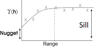
DHSA starts with geostatistics and variogram generation. I won’t go through this because there are plenty of reference out there on this. Typically a variogram look something like this:
The underlying principal of DHSA is “extension variance“, a method documented by Journel and Huijbregts (1978). There are a number of charts in this textbook, and one is given below:
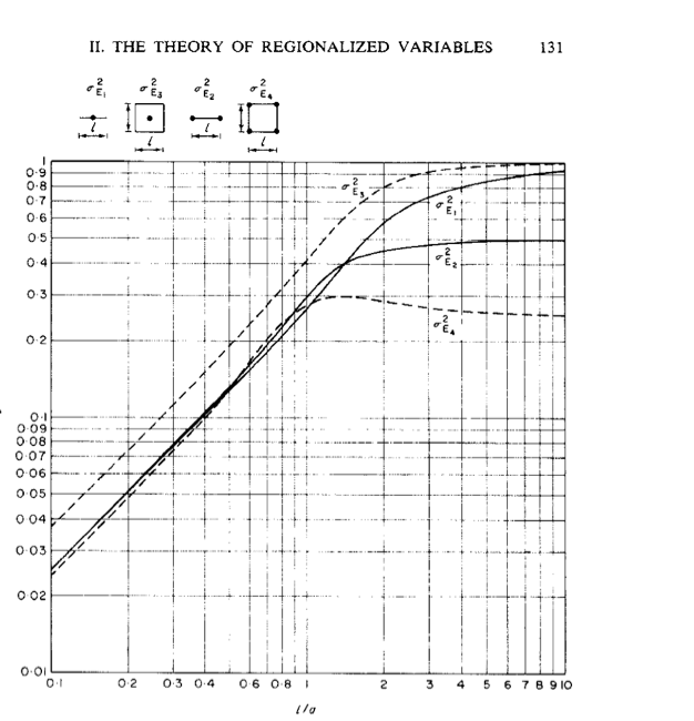
Journel, A.G., and Huijbregts, C.J., 1978: Mining Geostatistics, Academic Press, London.
DHSA uses the experimental variogram to extend the variance measured at a point to the variance within a larger block of specific dimensions surrounding the point. The estimation variance is the error made when assuming that the grade of the small volume, a drillhole is the true grade of a larger volume such as a mining block.
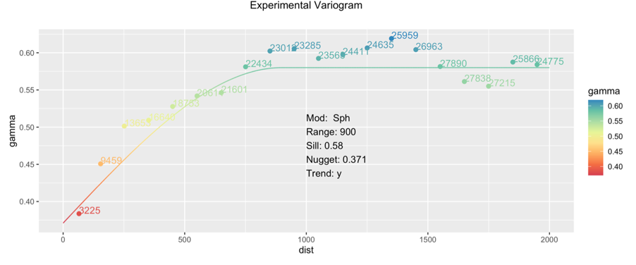
The chart contains an l/a ratio as x-axis. The y-axis is the extension variance. “l” refers to the range of your variogram, and “a” to a block size or for our application a drillhole spacing. The extension variance can be looked up from the chart, by calculating the ratio first (e.g. 300m (drillhole spacing) /900m (range) to give a l/a ration of 0.33. By looking up the chart, you get an extension variance of 0.12.
This extension variance is for a variogram with a nugget of zero, and a sill of 1.0. It needs to be applied to your own model. To do this you multiply 0.12 by the sill value of your model and add the nugget to get the of 0.441 for the variogram shown earlier.
Once the estimation variance is known for a given block size, it is a simple matter to calculate the estimation variance for a large area by dividing the single block estimation variance by the total number of blocks in the target area. This is known as the global estimation variance. To calculate the global estimation variance for different timeframes, the divisor is the number of blocks for 1 year multiplied by the number years.
The global estimation precision of the estimate is then calculated as 1.96 times the square root of the global estimation variance, divided by the mean which gives an error range with a confidence of 95%.
By completing the calculation at different block sizes you can generate a graph showing how precision changes over different spacings.
The advantage of the method is that DHSA can be conducted in a spreadsheet once the experimental variogram is defined compared to other methods such as conditional simulation which require more intense computations.
Leave a comment if you find this post useful.